Your First Analysis

PolyGenius is one flexible workflow, not a fixed pipeline. It is built from a small set of inter-linked modules — generate brings a PGS in, compute scores it against your genotypes, associate and evaluate relate or compare, visualize draws the result — plus workspace for configuration. You combine these modules to fit your research question; nothing forces you through one route.

library(dplyr)
## 
## Attaching package: 'dplyr'
## The following objects are masked from 'package:stats':
## 
##     filter, lag
## The following objects are masked from 'package:base':
## 
##     intersect, setdiff, setequal, union
library(PolyGenius)
workspace
## 
## ── PolyGenius workspace ────────────────────────────────────────────────────────
## Runtime context for generate, compute, associate, evaluate, and visualize.
## 
## Root /home/holstegelab-ggreen/.cache/R/PolyGenius
## Cores 1 (auto) · Memory Inf · Status yes · Verbosity info
## 
## › workspace$config configure root, cores, memory, verbosity, execution status
## › workspace$setup ✓ plink – gctb – prscs ✓ bigsnpr
## › workspace$catalogs reference panels, LD, liftover chains, genome builds
## › workspace$.internal execution engine internals
## 
## ℹ `workspace$config$update(root = ..., max.cores = ...)` to change settings

dplyr loads first because dplyr's own compute() generic would otherwise mask PolyGenius's compute module — the reverse order works too, but then compute$scores() needs the PolyGenius:: prefix to disambiguate, so loading dplyr first is the simpler habit.

One object holding where PolyGenius keeps its files and how much of your machine it's allowed to use — everything else reads its settings from here.

See Resources and Catalogs for how workspace resolves and caches everything external to your own data.

Bring in a model

The simplest PGS analysis applies a predefined score to your genotypes. generate gives you three ways in: retrieve a published score from the PGS Catalog, load a scoring file you already have on disk with generate$from.pgs.file(), or construct a PGS directly from your own variant table with PGS(variants = ..., name = ..., build = ..., ...) if neither of those fits.

models <- generate$from.pgs.catalog("PGS002280")
models
## <unnamed> PGSLibrary with 1 models
## # A tibble: 1 × 3
##   name      build       nvars
##   <chr>     <chr>       <int>
## 1 PGS002280 hg38/GRCh38    83
## ℹ generate$from.pgs.catalog() · v1.0.0 · 2026-10-02 12:14 · provenance()

"PGS002280" was already known here — finding one for your own trait means searching the PGS Catalog itself for the phenotype you care about; its page gives you the ID this function expects.

A model and a cohort must share a genome build. That is checked when the study object is built, not silently coerced — a mismatch is fixed with a separate liftover() call beforehand.

See Getting a Model In and Out for the other two routes and for writing a model back out.

Attach it, then the workflow at a glance

A PolyGeniusStudy couples a set of PGS models (narrowed into a library it owns, data$library) to a cohort's genotype pointer (GenotypeSource) and sample-level data (phenotypes, covariates) into one object. That coupling matters because every downstream step — compute$scores(), associate$*(), evaluate$*(), visualize$*() — takes this one object as its first argument and writes its output back onto it, so scores, associations, evaluations and derived signals all accumulate on the same hub.

See A PolyGenius Study for what else lives on this object, what shape pheno needs to be in (values are matched to samples by their IDs, or by position when they carry none), and how subsetting it behaves.

data <- PolyGeniusStudy(
  name      = "cohort",
  library   = models,
  genotypes = GenotypeSource(path = "...", format = "pfile", build = "GRCh38", name = "cohort"),
  samples   = list(phenotypes = pheno)
)

To make the rest of this page runnable, data below actually holds a small synthetic cohort — genotypes simulated at PGS002280's own variant positions, phenotypes drawn to match ROSMAP's own published rates (56.72% demented, 66.98% female) — not real patient records. Swap in your own GenotypeSource and pheno to run this on real data.

From here, four steps chain onto the same data object.

1. Relatedness

Every regression below assumes its observations are independent. Related samples break that assumption silently — they inflate your confidence in a result rather than raising an error — and related samples also distort population-structure PCs if you leave them in.

data$sample.pairs$kinship <- compute$relatedness$kinship(data, degree = 2, variants = background.variants)
data$samples$unrelated    <- compute$relatedness$prune(data, degree = 2)
data                      <- data[unrelated, ]

degree = 2 is both the function default and a conventional cutoff — it flags duplicates through second-degree relatives (siblings are first-degree; half siblings and grandparent-grandchild are second) and is a reasonable starting point for most cohorts. prune()'s key argument defaults to "kinship", so — called here with the same degree = 2 — it reads the matrix already stored at data$sample.pairs$kinship instead of recomputing it from genotypes. It only recomputes when no matrix is found at key. A stored matrix computed at a coarser cut point than requested is refused, because the pairs in between were never computed.

variants supplies the marker set kinship is estimated from — a real cohort's genotyping array covers far more variants than any one PGS scores on, so PolyGenius defaults to the curated, genome-wide common20k variant space here rather than reusing the PGS's own handful of variants; background.variants is this walkthrough's small in-memory stand-in for that marker set, built earlier alongside the synthetic cohort.

2. Score computation

data$scores$X        <- compute$scores(data, maf.thr = 0.01)
data$scores$X.scaled <- compute$standardize(data)

0.01 is a common working choice, not a package default — PolyGenius applies no frequency filter unless you ask for one. compute$standardize() defaults to standardizing whichever layer is named X, which is why the raw scores above are assigned there rather than to an arbitrary name. It turns a scale-dependent raw sum into a per-SD effect, the form you almost always want to report.

3. Population structure

This has to come after relatedness pruning, and that order is a statistical requirement, not a style choice: principal components estimated on a sample that still contains families are pulled toward those families, distorting the very axes you are about to compute, rather than describing ancestry cleanly.

Separately — and this is why you want PCs as covariates at all, not why they must come after pruning — the GWAS behind your score ran in some source population, and if your cohort's ancestry varies, that axis correlates with both the score and, often, the outcome; including these PCs as covariates absorbs that confounder in this regression. It does not make the score itself transferable across ancestries — a European-discovery score stays less accurate in a more diverse or admixed cohort no matter how many PCs you add, which is a separate, actively studied problem this page doesn't cover.

data$samples$PCA <- compute$populationStructure(data, npcs = 5, variants = background.variants)

npcs = 5 is the function's own default and enough to absorb the broad ancestry axes most cohorts need; a cohort with finer population structure may need more. variants plays the same role as in the relatedness step above — its own default also resolves a downloaded reference panel.

4. Association

associate$regression() answers one question — how strongly does a predictor relate to an outcome, adjusted for covariates — across outcome shapes it detects automatically: two-category fits logistic regression, continuous fits linear regression, a time-to-event outcome wrapped in surv(time=, event=) fits a Cox model, or a Fine-Gray competing-risk model when competing.event= is also named.

The outcomes below (demented, dementia diagnosis; braaksc/ceradsc, two neuropathology staging scores) are the kind of columns a real dementia cohort has — swap in whatever phenotype and covariate columns your own study has; nothing about the call itself is dementia-specific. braaksc and ceradsc are ordinal staging scores with more than two levels, so auto-detection fits them as continuous outcomes by ordinary least squares — a common approximation in neuropathology PGS work, not evidence that ordinal levels are modelled as such; PolyGenius has no proportional-odds or ordinal-logistic family to opt into instead.

assoc <- associate$regression(
  data,
  outcomes     = c(demented, braaksc, ceradsc),
  scores.layer = X.scaled,
  covariates   = c(sex, age.exit, PCA)
)
data$associations <- assoc
assoc
## 
## ── PolyGenius association ──────────────────────────────────────────────────────
## 
##     outcome predictor      term term.type  estimate         se      lower
##      <char>    <char>    <char>    <char>     <num>      <num>      <num>
## 1: demented PGS002280 PGS002280      main 0.5794942 0.13276980 0.31927020
## 2:  braaksc PGS002280 PGS002280      main 0.3421352 0.08200294 0.18074117
## 3:  ceradsc PGS002280 PGS002280      main 0.1355329 0.05315427 0.03091737
## 28 variable(s) not shown: [upper <num>, statistic <num>, pval <num>, adj.pval <num>, n <num>, stratum <char>, adj.family.id <int>, effect.scale <char>, test <char>, outcome.type <char>, ...]
## 
## Schemas: glm, lm • Families: glm, lm • 3 result rows • 3 fits
## 
## • Artifacts:
##   • prediction.grid: <table 150 × 4> predictor.value, fitted.value, se, .fit
## ℹ associate$regression() · v1.0.0 · 2026-10-02 12:14 · provenance()

associate estimates an effect; evaluate compares candidate models.

Which association fits your question is its own decision — see Choosing an Association Analysis. From there: Regression Associations covers subgroups and comparisons within the call above; Survival Associations covers surv() and competing risks; Mediation splits an effect into a direct and an indirect part; Single-Variant Associations runs the same shape of analysis per-variant instead of per-score; Meta-Analysis pools results like assoc across cohorts without moving individual-level data.

Plot and save

assoc mixes two regression families here — demented fit as logistic, braaksc/ceradsc as linear — and forest() plots one family at a time, so it needs a filter first:

visualize$associations$forest(assoc %>% filter(family == "glm"))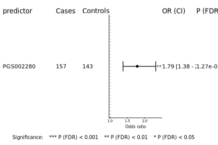

Every table and whisker value here traces back to a column already on assoc$results, with no new statistic computed from raw data. The one built-in exception is display scale: for a logistic, Cox, or competing-risk fit, the plot shows an odds ratio, hazard ratio, or subdistribution hazard ratio (respectively — a competing-risk model answers a different question from a Cox model, so its ratio isn't interchangeable with one) by exponentiating the stored log-scale estimate. What you see on the axis is not literally a stored column, but it is always a fixed, documented transform of one.

One warning worth having before you hit it yourself: what comes back is a patchwork plot nested two levels deep. + theme(...) only touches the last-added top-level element — the legend strip — and visibly does almost nothing to the actual plot panels. & theme(...) recurses into every nested panel and actually restyles the whole figure. Use &, not +, to theme this plot:

visualize$associations$forest(assoc %>% filter(family == "glm")) & theme(text = element_text(family = "sans"))

ggplot2::ggsave("cohort-forest.png", visualize$associations$forest(assoc %>% filter(family == "glm")))

There is no package-provided save helper — plain ggsave() works directly here, once you either library(ggplot2) or call it namespaced as above; PolyGenius uses ggplot2 internally but does not attach it for you. Other visualize$* calls return other types (a Heatmap, a list of plots), which need different handling; see Plots.

savePolyGenius(data, "cohort-analysis.pgd")

This writes the whole study — model library, sample tables, the kinship matrix on $sample.pairs, and everything accumulated on $scores, $associations, $evaluations, $signals and $uns — into one portable .pgd file that loadPolyGenius() reconstructs in full. See Persistence and the Backbone for what the file physically contains.

Where to go next

Choosing an Association Analysis and its chapters cover the other shapes an association can take. If no published score fits your GWAS or your ancestry, building your own PGS instead of importing one starts at GWAS Sources.